
Excel 2010 -
Formatting Cells

Excel 2010
Formatting Cells

search
menu
/en/excel2010/modifying-columns-rows-and-cells/content/
Spreadsheets that have not been formatted can be difficult to read. Formatted text and cells can draw attention to specific parts of the spreadsheet and make the spreadsheet more visually appealing and easier to understand.
In Excel, there are many tools you can use to format text and cells. In this lesson, you will learn how to change the color and style of text and cells, align text, and apply special formatting to numbers and dates.
Many of the commands you will use to format text can be found in the Font, Alignment, and Number groups on the Ribbon. Font commands let you change the style, size, and color of text. You can also use them to add borders and fill colors to cells. Alignment commands let you format how text is displayed across cells both horizontally and vertically. Number commands let you change how selected cells display numbers and dates.
Optional: You can download this example for extra practice.
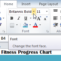
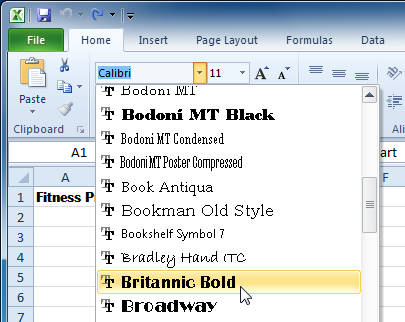 Changing the font
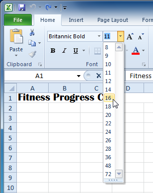 Changing the font size
You can also use the Grow Font and Shrink Font commands to change the size.
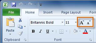 The Grow Font and Shrink Font commands
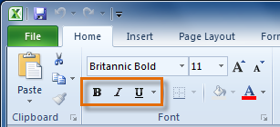 The Bold, Italic, and Underline commands
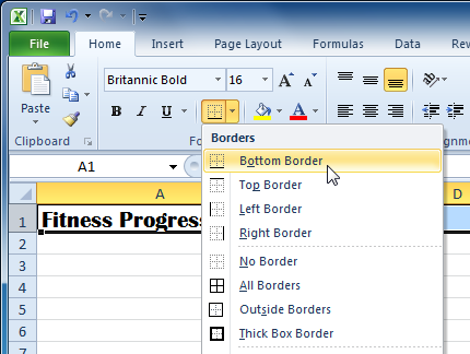 Adding a border
You can draw borders and change the line style and color of borders with the Draw Borders tools at the bottom of the Borders drop-down menu.
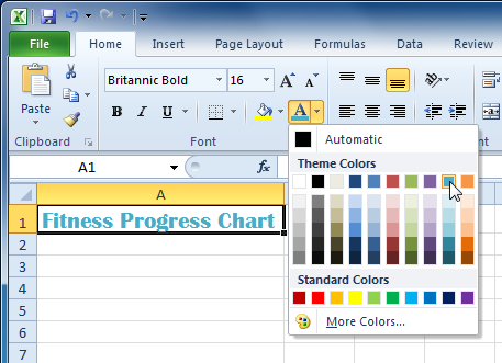 Adding a font color
Your color choices are not limited to the drop-down menu that appears. Select More Colors at the bottom of the menu to access additional color options.
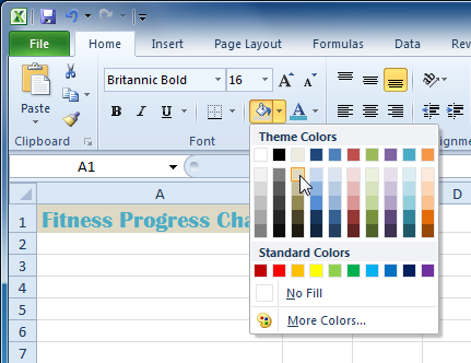 Adding a fill color
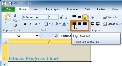 Aligning Text Left
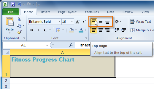 Top Aligning Text
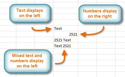
By default, numbers align to the bottom-right of cells, while words and letters align to the bottom-left of cells.
If you want to copy formatting from one cell to another, you can use the Format Painter command on the Home tab. When you click the Format Painter, it will copy all of the formatting from the selected cell. You can then click and drag over any cells you want to paste the formatting to.
Watch the video below to learn two different ways to use the Format Painter.
One of Excel's most useful features is its ability to format numbers and dates in a variety of ways. For example, you might need to format numbers with decimal places, currency symbols ($), or percent symbols (%).
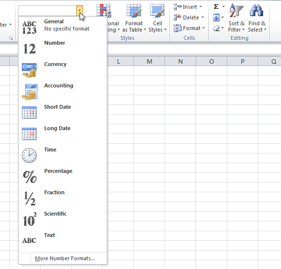
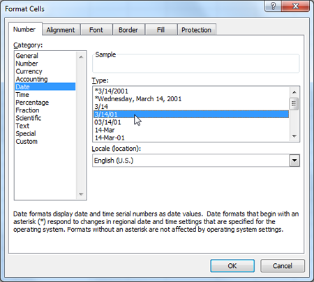
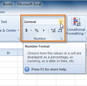 Accessing Number Format commands
Click the buttons in the interactive below to learn about the different number formats.
You can easily customize any format in More Number Formats.
For example, you can change the U.S. dollar sign to another currency sign, have numbers display commas, and change the number of displayed decimal places.
Text formats numbers as text, meaning what you enter into the cell will appear exactly as you wrote it. Excel defaults to this setting if a cell contains both text and numbers.
Scientific formats numbers in scientific notation.
For example, if you enter 140000 into the cell, then the cell will display the number as 1.40E+05.
Note: By default, Excel will format the cell in scientific notation if it is a large integer. If you do not want Excel to format large integers with scientific notation, use the Number format.
Fraction formats numbers as fractions separated by the forward slash.
For example, if you enter 1/4 into the cell, the cell will display the number as 1/4. If you enter 1/4 into a cell that is formatted as General, the cell will display the number as a date, 4-Jan.
Percent formats numbers with decimal places and the percent sign.
For example, if you enter 0.75 into the cell, the cell will display the number as 75.00%.
Long Date formats numbers as Weekday, Month DD, YYYY.
For example, it would appear in this format: Monday, August 01, 2010.
Time formats numbers as HH/MM/SS and notes AM or PM.
For example, it would appear in this format: 10:25:00 AM.
Short Date formats numbers as M/D/YYYY.
For example, August 8th, 2010, would be 8/8/2010.
Accounting formats numbers as monetary values like the Currency format, but it also aligns currency symbols and decimal places within columns. This format will make it easier for you to read long lists of currency figures.
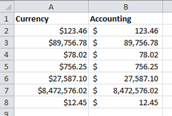
Currency formats numbers as currency with a currency symbol.
For example, if you enter 4 into the cell, the cell will display the number as $4.00.
Number formats numbers with decimal places.
For example, if you enter 4 into the cell, the cell will display the number as 4.00.
General is the default format for any cell. When you enter a number into the cell, Excel will guess the number format that is most appropriate.
For example, if you enter 1-5, the cell will display the number as a Short Date, 1/5/2010.
/en/excel2010/saving/content/