By default, the cells of every new spreadsheet are always the same size. Once you begin entering information into your spreadsheet, it's easy to customize rows and columns to better fit your data.
In this lesson, you'll learn how to change the height and width of rows and columns, as well as how to insert, move, delete, and freeze them. You'll also learn how to wrap and merge cells.
Watch the video below to learn more about modifying cells in Google Sheets.
Working with columns, rows, and cells
Every row and column of a new spreadsheet is always set to the same height and width. As you begin to work with spreadsheets, you will find that these default sizes are not always well-suited to different types of cell content.
To modify column width:
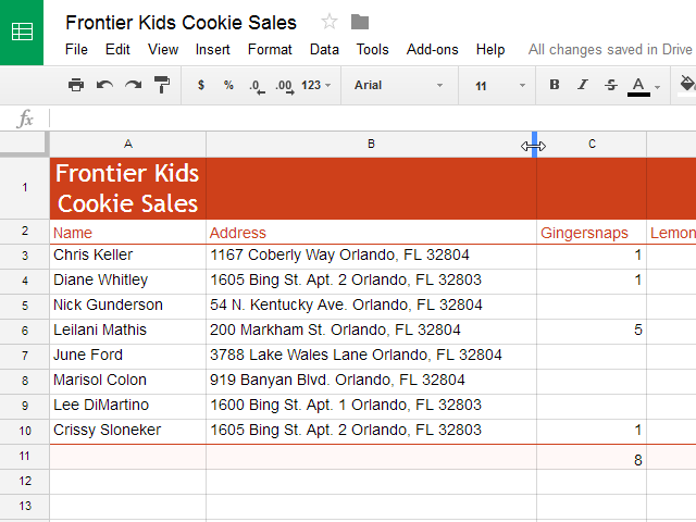
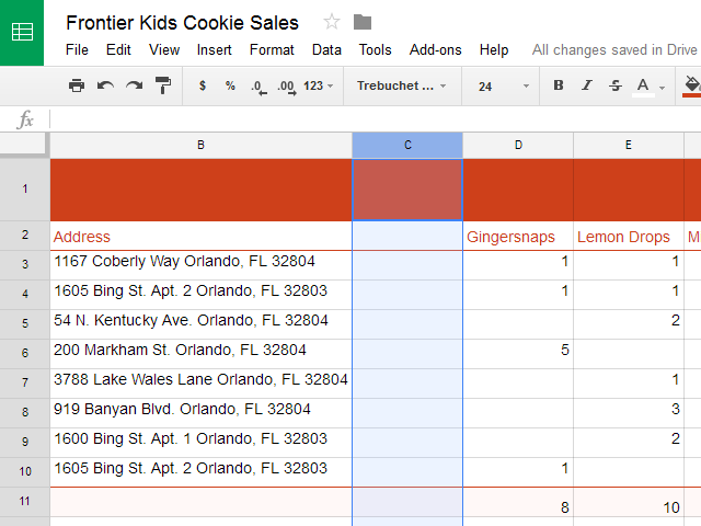
In our example below, some of the content in column B is too long to be displayed. We can make all of this content visible by changing the width of column B.
Hover the mouse over the line between two columns. The cursor will turn into a double arrow.
Click and drag the column border to the right to increasecolumn width. Dragging the border to the left will decrease column width.
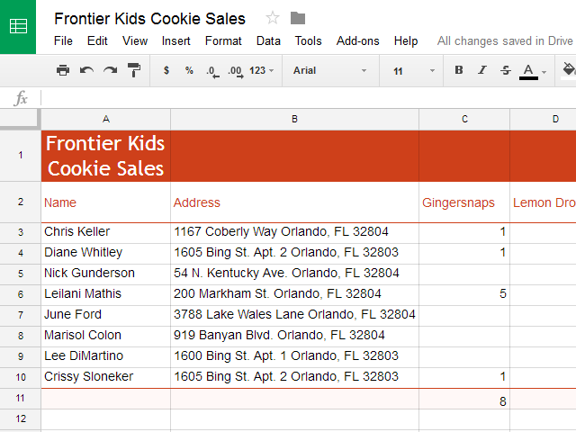
Release the mouse when you are satisfied with the new column width. All of the cell content is now visible.
To autosize a column's width:
The autosizing feature will allow you to set a column's width to fit its content automatically.
Hover the mouse over the line between two columns. The cursor will turn into a double arrow.
Double-click the mouse.
The column's width will be changed to fit the content.
To modify row height:
You can make cells taller by modifying the row height. Changing the row height will create additional space in a cell, which often makes it easier to view cell content.
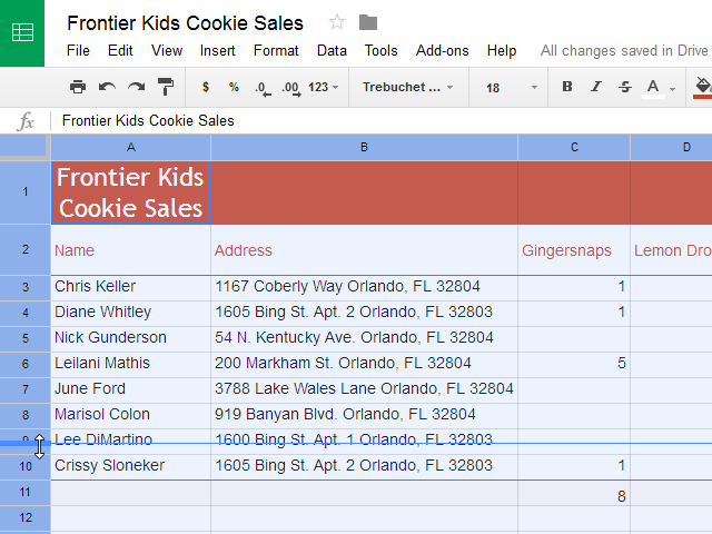
Hover the mouse over the line between two rows. The cursor will turn into a double arrow.
Click and drag the row border down to increase the height. Dragging the border up will decrease the row height.
Release the mouse when you are satisfied with the new row height.
To modify all rows or columns:
Rather than resizing rows and columns individually, you can modify the height and width of every row and column in a spreadsheet at the same time using the Select All button. This method allows you to set a uniform size for the spreadsheet's rows and columns. In our example, we'll set a uniform row height.
Click the Select All button just below the formula bar to select every cell in the spreadsheet.
Hover the mouse over the line between two rows. The cursor will turn into a double arrow.
Click and drag the row border to modify the height.
Release the mouse when you are satisfied with the new row height for the spreadsheet.
Inserting, deleting, and moving rows and columns
After you've been working with a spreadsheet for a while, you may find that you want to add new columns or rows, delete certain rows or columns, or even move them to a different location in the spreadsheet.
To insert a column:
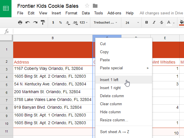
Right-click a column heading. A drop-down menu will appear. There are two options to add a column. Select Insert 1 left to add a column to the left of the current column, or select Insert 1 right to add a column to the right of the current column.
The new column will be inserted into the spreadsheet.
To insert a row:
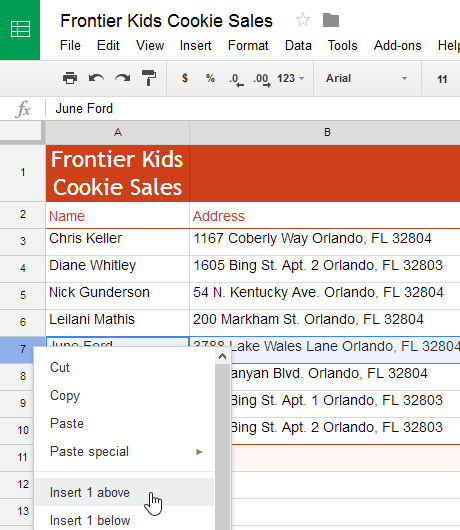
Right-click a row heading. A drop-down menu will appear. There are two options to add a row. Select Insert 1 above to add a row above the current row, or select Insert 1 below to add a row below the current row.
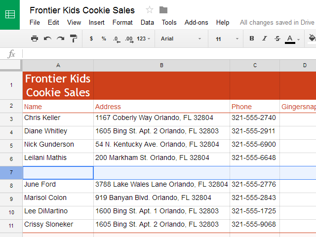
The new row will be inserted into the spreadsheet.
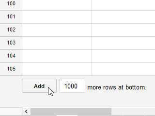
If you need to add more than one row at a time, you can scroll to the bottom of the spreadsheet and click the Add button. By default, this will add 1000 new rows to your spreadsheet, but you can also set the number of rows to add in the text box.
To delete a row or column:
It's easy to delete any row or column you no longer need in your spreadsheet. In our example, we'll delete a row, but you can delete a column in the same way.
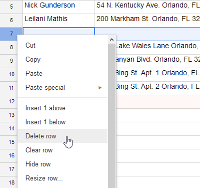
Select the row you want to delete.
Right-click the row heading, then select Delete row from the drop-down menu.
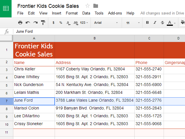
The rows below the deleted row will shift up to take its place. In our example, row 8 is now row 7.
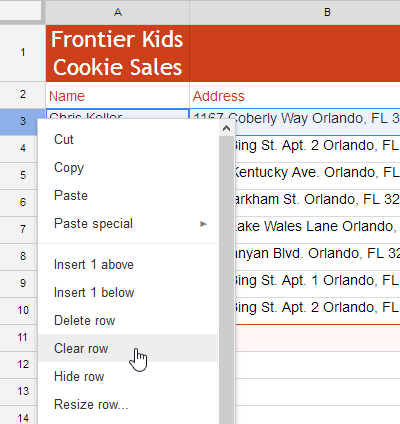
There's a difference between deleting a row or column and simply clearingits contents. If you want to remove the content of a row or column without causing the others to shift, right-click a heading, then select Clear row or Clear column.
To move a row or column:
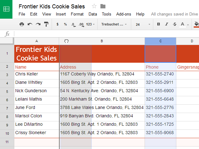
Sometimes you may want to move a column or row to make it more accessible in your spreadsheet. In our example, we'll move a column, but you can move a row in the same way.
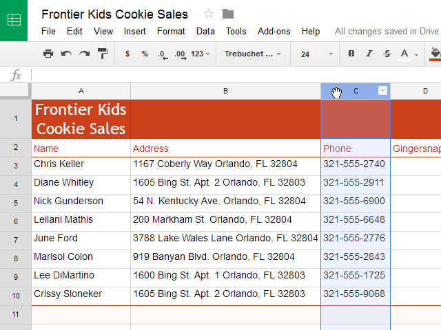
Select the column you want to move, then hover the mouse over the column heading. The cursor will become a hand icon.
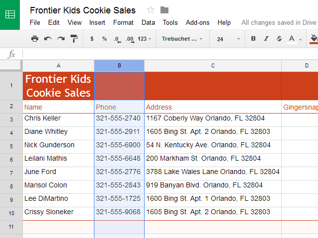
Click and drag the column to its desiredposition. An outline of the column will appear.
Release the mouse when you are satisfied with the new location.
Wrapping text and merging cells
Whenever you have too much cell content to be displayed in a single cell, you may decide to wrap the text or merge the cell rather than resize a column. Wrapping the text will automatically modify a cell's row height, allowing the cell contents to be displayed on multiple lines. Merging allows you to combine a cell with adjacent empty cells to create one large cell.
To wrap text:
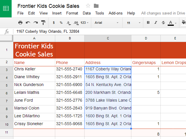
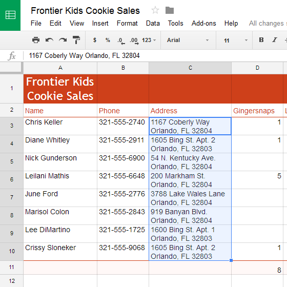
Select the cells you want to wrap. In this example, we're selecting cell range C3:C10.
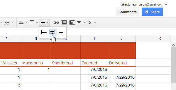
Open the Text wrapping drop-down menu, then click the Wrap button.
The cells will be automatically resized to fit their content.
To merge cells:
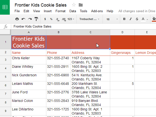
Select the cells you want to merge. In this example, we're selecting cell range A1:C1.
Select the Merge cells button.
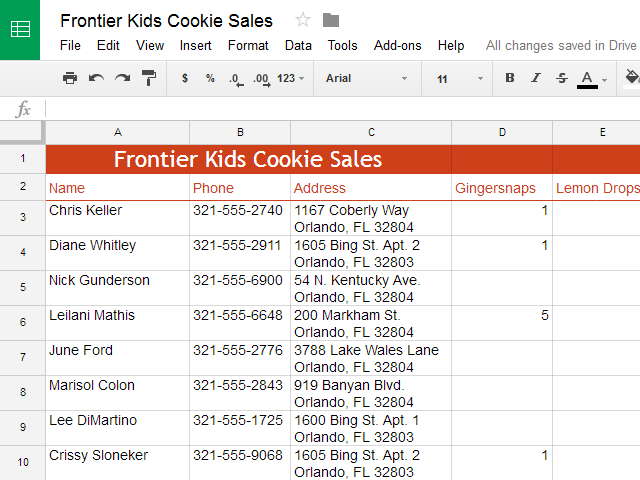
The cells will now be merged into a single cell.
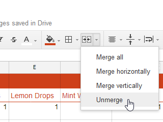
To unmerge a cell, click the drop-down arrow next to the Merge cells button, then select Unmerge from the drop-down menu.
Freezing rows and columns
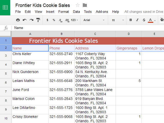
When working with large spreadsheets, there will be times when you'll want to see certain rows or columns all the time, especially when using header cells as in our example below. By freezing rows or columns in place, you'll be able to scroll through your spreadsheet while continuing to see the header cells.
To freeze a row:
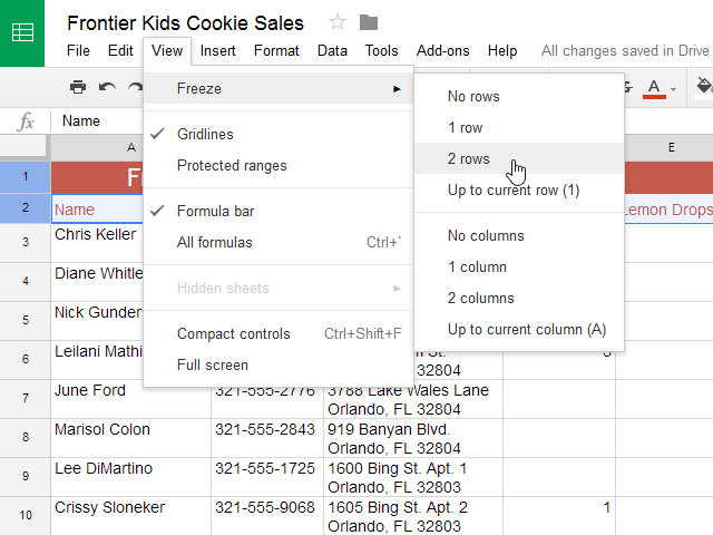
Locate the row or rows you want to freeze. In this example, we'll freeze thetop two rows. Note: You do not need to select the rows you want to freeze.
Click View in the toolbar. Hover the mouse over Freeze, then select the desired number of rows to freeze from the drop-down menu.
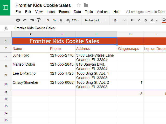
The top two rows are frozen in place. You can scroll down your worksheet while continuing to view the frozen rows at the top.
To freeze a column:
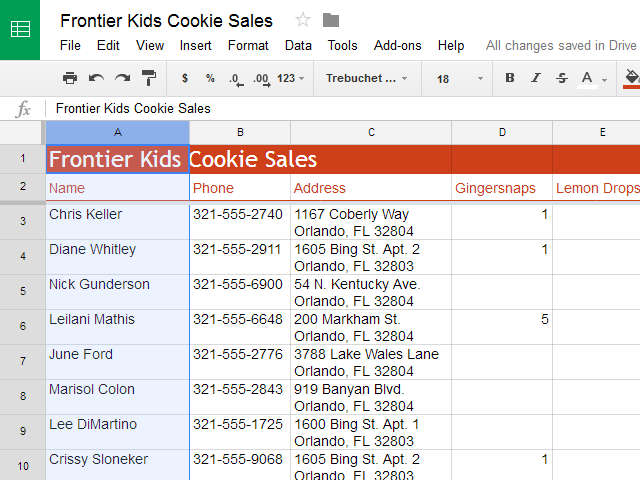
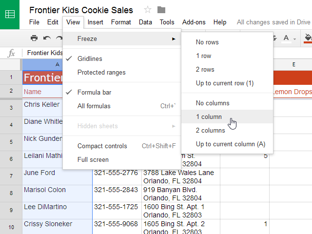
Locate the column or columns you want to freeze. In this example, we'll freeze theleftmost column. Note: You do not need to select the columns you want to freeze.
Click View in the toolbar. Hover the mouse over Freeze, then select the desired number of columns to freeze from the drop-down menu.
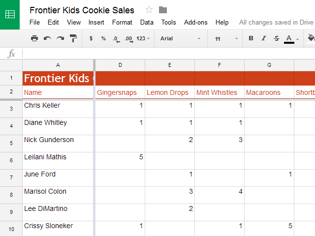
The leftmost column is now frozen in place. You can scroll across your worksheet while continuing to view the frozen column on the left.
To unfreeze rows, click View, hover the mouse over Freeze, then select No rows. To unfreeze columns, click View, hover the mouse over Freeze, then select No columns.
Challenge!
Open our example file. Make sure you're signed in to Google, then click File > Make a copy.
Change the row height of all of the rows to be smaller.
Merge cells A1:I1.
Insert a row below row 11 and type your name in the first cell.
Delete row 7. This row contains the name Ben Mathis.
Insert a column between columns G and H and type Total Quantity as the column header.
Select cells A2:J2, change them to wrap text, and center align them.
Freeze the top two rows.
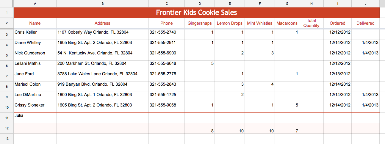
When you're finished, your spreadsheet should look something like this: