Excel Tips: A Trick for Finding Inconsistent Data

Lesson 18: A Trick for Finding Inconsistent Data

/en/excel-tips/what-are-named-ranges/content/

A trick for finding inconsistent data

With larger spreadsheets, it can be difficult to find all of the inconsistencies in your data. In this lesson, we'll show you a shortcut that makes it much easier.

Watch the video below to learn a trick for finding inconsistent data.

Understanding the problem

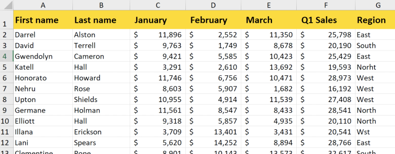
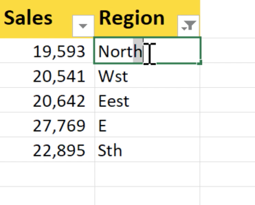
In the example below, we have a list of salespeople, and each one falls into one of four regions (in column G): North, South, East, or West. If you look closely, you may notice that the regions for Katell Hall and Illana Erickson are misspelled. This could cause problems with certain formulas or PivotTables, so it's important to correct these errors.

It's easy enough to fix two errors, but what if there are more? In our spreadsheet, there are hundreds of rows, so it would take a long time to check each cell for errors. Luckily, there is an easier way to find them all.

Steps

Let's go over the steps to find and fix the inconsistencies...

The key to finding the inconsistencies is to create a filter. The filter will allow you to see all of the unique values in the column, making it easier to isolate the incorrect values. In our example, the Region column should only contain the values North, South, East, and West, so any other values will need to be fixed.

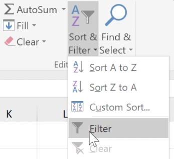
On the Home tab, go to Sort & Filter > Filter. If your worksheet already has filters, you can skip this step.
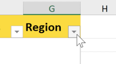
Click the filter drop-down arrow in the desired column.
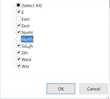
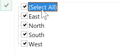
A drop-down menu will appear, showing a list of all of the unique values in the column. Deselect all of the correct values, leaving all of the incorrect values selected. In our example, we will deselect North, South, East, and West. When you're done, click OK.
The spreadsheet will now be filtered to only show the incorrect values. In our example, there were only a few errors, so we'll fix them manually by typing the correct values for each one.
Click the column's filter drop-down arrow again and make sure all of the values listed are correct. When you're done, click Select All, then click OK to show all of the rows.

That's it! All of the values in the Region column are now consistent.

In Excel, details matter. If you have minor inconsistencies in your data, it can cause major problems later on.

Moving into Excel functions...

Now we'll move into more Excel functions, starting with VLOOKUP. These lessons are structured a little differently, but we think you'll find them just as helpful!