
Excel 2010 -
Creating Complex Formulas

Excel 2010
Creating Complex Formulas

search
menu
/en/excel2010/printing/content/
Excel is a spreadsheet application that can help you calculate and analyze numerical information for household budgets, company finances, inventory, and more. To do this, you need to understand complex formulas.
In this lesson, you'll learn how to write complex formulas in Excel following the order of operations. You will also learn about relative and absolute cell references, as well as how to copy and fill formulas containing cell references.
Simple formulas have one mathematical operation, such as 5+5. Complex formulas have more than one mathematical operation, such as 5+5-2. When there is more than one operation in a formula, the order of operations tells us which operation to calculate first. To use Excel to calculate complex formulas, you'll need to understand the order of operations.
Optional: You can download this example for extra practice.
Excel calculates formulas based on the following order of operations:
A mnemonic that can help you remember the order is Please Excuse My Dear Aunt Sally.
The following example demonstrates how to use the order of operations to calculate a formula:
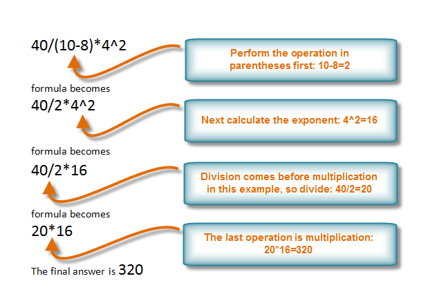 Order of Operations example
In this example, we'll review how Excel will calculate a complex formula using the order of operations. The selected cell will display the percent of total Pete Lily seeds sold that were white.
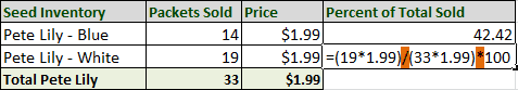 Order of Operations Excel example
Based on this complex formula, the result will show that 57.58% of the total Pete Lily seeds sold were white. You can see from this example that it is important to enter complex formulas with the correct order of operations. Otherwise, Excel will not calculate the results accurately.
In this example, we'll use cell references in addition to actual values to create a complex formula that will add tax to the nursery order.
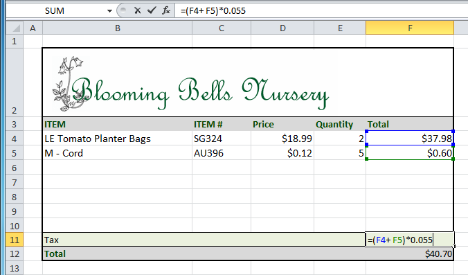 Typing a formula
 Result in F11
Excel will not always tell you if your formula contains an error, so it's up to you to check all of your formulas. To learn how to do this, you can read the Double-Check Your Formulas lesson from our Excel Formulas tutorial.
In order to maintain accurate formulas, it is necessary to understand how cell references respond when you copy or fill them to new cells in the worksheet.
Excel will interpret cell references as either relative or absolute. By default, cell references are relative references. When copied or filled, they change based on the relative position of rows and columns. If you copy a formula (=A1+B1) into row 2, the formula will change to become (=A2+B2).
Absolute references, on the other hand, do not change when they are copied or filled and are used when you want the values to stay the same.
Relative references can save you time when you're repeating the same type of calculation across multiple rows or columns.
In the following example, we're creating a formula with cell references in row 4 to calculate the total cost of the electric bill and water bill for each month (B4=B2+B3). For the upcoming months, we want to use the same formula with relative references (C2+C3, D2+D3, E2+E3, etc.). For convenience, we can copy the formula in B4 into the rest of row 4, and Excel will calculate the value of the bills for these months using relative references.
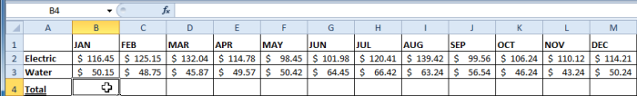 Selecting cell B4
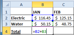 Entering formula into B4
 Result in B4
 Values calculated in C4:M4
There may be times when you do not want a cell reference to change when copying or filling cells. You can use an absolute reference to keep a row and/or column constant in the formula.
An absolute reference is designated in a formula by the addition of a dollar sign ($) before the column and row. If it precedes the column or row (but not both), it's known as a mixed reference.
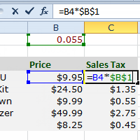
In the below example, we want to calculate the sales tax for a list of products with varying prices. We'll use an absolute reference for the sales tax ($B$1) because we do not want it to change as we are copying the formula down the column of varying prices.
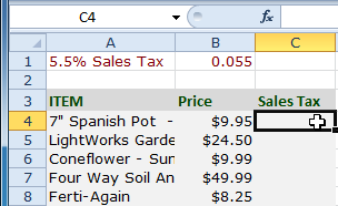 Selecting cell C4
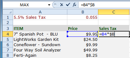 Entering formula
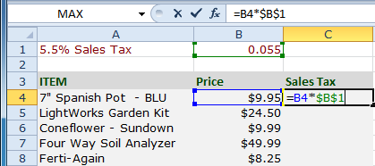 Entering formula
 Result in C4
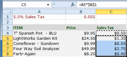 Values calculated in C5:C8
When writing a formula, you can press the F4 key on your keyboard to switch between relative and absolute cell references, as shown in the video below. This is an easy way to quickly insert an absolute reference.
/en/excel2010/working-with-basic-functions/content/