Lesson 23: Invoice, Part 4: More Shipping Options
/en/excelformulas/invoice-part-3-fix-broken-vlookup/content/

"I know, I know. It's always something right? Anyway, we're going to start offering some new shipping options.
I put all of the options into a new worksheet. I remembered that you were able to use that VLOOKUP function to pull in the product name and price. Do you think you could do the same thing for the shipping option?"
This lesson is part 4 of 5 in a series. You can go to Invoice, Part 1: Free Shipping if you'd like to start from the beginning.
Our spreadsheet
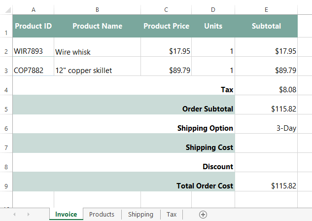
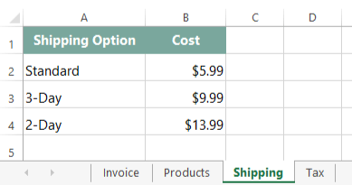
Once you've downloaded our spreadsheet, open the file in Excel or another spreadsheet application. It looks similar to our spreadsheet from the previous lesson, but now there are some new rows for the shipping options, along with a new Shipping worksheet with different shipping options and costs.
What are we trying to do?
We'll need to use the Shipping Option (in cell E6) to automatically pull in the Shipping Cost for cell E7. We can use a VLOOKUP function to do this automatically.
If you've never used VLOOKUP before, you can go to Invoice, Part 2: Using VLOOKUP to learn the basics.
Writing the function
This VLOOKUP function will actually be similar to the VLOOKUP function we created in Invoice, Part 2: Using VLOOKUP. We'll start by typing the equals sign (=), followed by the function name and an open parenthesis:
=VLOOKUP(
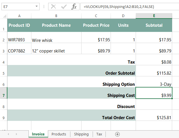
Next, we'll add our arguments. The first argument tells VLOOKUP what to search for. In our example, it will search for the Shipping Option, which we will be typing in cell E6 of our Invoice.
=VLOOKUP(E6
The second argument tells VLOOKUP where to look for the value in our first argument. In our example, that's in the Shipping worksheet, in cell range A2:B4.
We'll include some extra rows in the cell range in case more shipping options are added later.
=VLOOKUP(E6, Shipping!A2:B10
Finally, we'll add our third and fourth arguments. In this example, the Shipping Cost is in column B (the second column), so our third argument is 2. And because we're only looking for exact matches, the fourth argument is FALSE.
=VLOOKUP(E6, Shipping!A2:B10, 2, FALSE)
Type the formula into cell E7 of the Invoice and press Enter to see the result.
If you typed the formula correctly, the correct shipping price should appear: $9.99. If you want to make sure your formula is working correctly, change the Shipping Option in cell E6 from 3-Day to 2-Day. The Shipping Cost should change from $9.99 to $13.99.
Be sure to type the shipping option exactly as it appears in the worksheet, or the VLOOKUP function won't work correctly.

"Nice work here! But…I just remembered that we'll still be offering free standard shipping on orders over $100.
So if shoppers spend at least $100, they should get a credit for the cost of standard shipping ($5.99) toward their total order cost. Maybe you could just modify the IF function you added before to do this automatically."
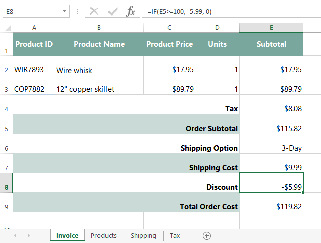
As you may remember from Invoice, Part 1: Free Shipping, we used the IF function to change the shipping cost to $0 if the cost of the order was at least $100. This time, we'll do it a bit differently: If the order is at least $100, we'll give them a credit of $5.99, which is the cost of standard shipping. This means standard shipping will be free, and the more expensive shipping options will also get a discount of $5.99.
Just like before, our new formula will look at the Order Subtotal in cell E5 to see if the value is greater than or equal to $100, so our first argument will be E5>=100.
=IF(E5>=100
The second argument looks to see if the statement in the first argument is true. If it's true, they'll receive a credit for the cost of standard shipping (5.99). Since the credit will be subtracted from the total order cost, we'll make it a negative number: -5.99.
=IF(E5>=100,-5.99
The third argument looks to see if the statement in the first argument is false. If it's false, they won't receive the $5.99 shipping credit. This means our third argument will be 0 (zero). We'll also add a close parenthesis after the last argument. Here's our new IF function:
=IF(E5>=100, -5.99, 0)
When you press Enter, the correct discount should appear in cell E8.
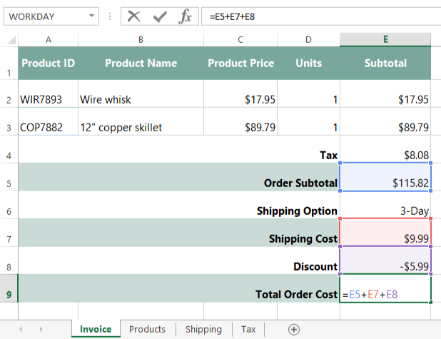
If we look at the formula that calculates the Total Order Cost in cell E9, we can calculate the total value of Order Subtotal, Shipping Cost, and Discount. We'll simply add all three values; since the Discount is a negative number, that value will be subtracted from the Total Order Cost.
OK—our formulas look good. Let's send this back!

"Perfect-a-mundo! Thanks as always! I don't know what we'd do without you!
I really appreciate your help—our invoice is working like a well-oiled machine!"
If you'd like to continue on to the next part in this series, go to Invoice, Part 5: Data Validation.
/en/excelformulas/invoice-part-5-data-validation/content/